January 17, 2017
OSTMap – Open Source Tweet Map
Research
It is often necessary to build a proof of concept to show the ease and feasibility of Big Data to customers / project promoters or colleagues. With OSTMap (Open Source Tweet Map) mgm partners with ScaDS to prove that it is possible to accomplish a lot with the right choice of technologies in a short time frame.
But first, what is OSTMap? OSTMap enables the user to view live, geo-tagged tweets of the last hours on a map, search all collected tweets by a term or user name and view the amount of incoming tweets per minute distinguished by language as a graph. OSTMap covers several important areas of a typical big data PoC projects: scalability, stream processing and ingest of incoming data, batch processing of stored data, near real-time queries and visualization of the data.
Project Setup
- Six Weeks
- Six Students
- 10h/week each
- No experience using Big Data technologies and concepts
- 2h of consultation per week with Big Data experts of ScaDS and mgm
To ensure that we will finish with a result development was done iteratively using the walking skeleton approach which allowed us to increase the feature set constantly even with a strict deadline.
“A Walking Skeleton is a tiny implementation of the system that performs a small end-to-end function. It need not use the final architecture, but it should link together the main architectural components. The architecture and the functionality can then evolve in parallel.”
Alistair Cockburn
Results
The OSTMap website is divided into four parts.
The term search is shown in the following figure. It is capable of basic searches (exact and prefix match) regarding users, single terms and hashtags. It is the only part of OSTMap which currently grants access to tweets older than one day.
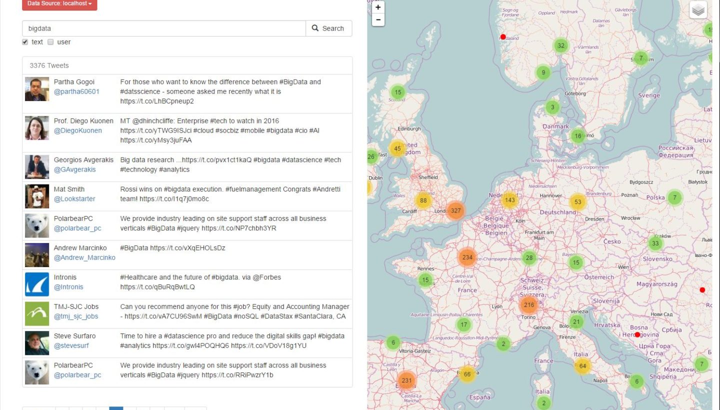
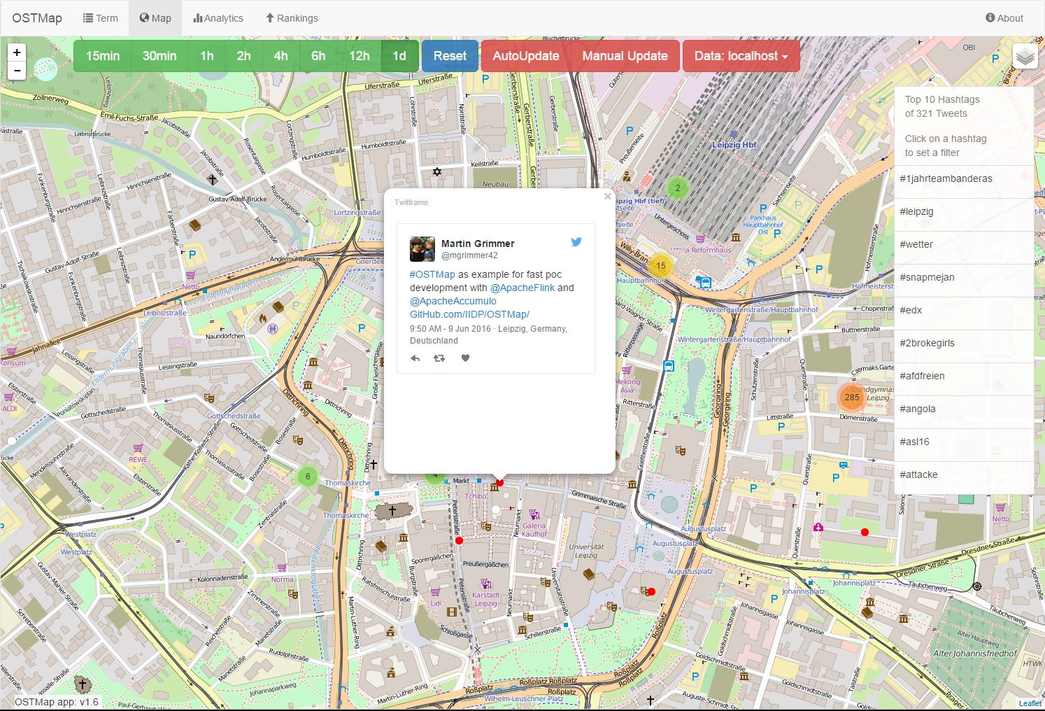
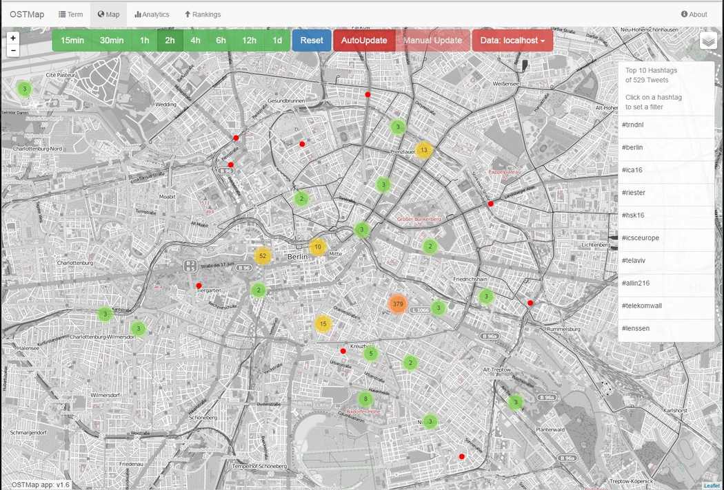
In the next two figures you can see the map search. It aggregates tweets for the chosen region and determines the top hashtags of the map view. By clicking on an aggregated bubble one is zooming in. At the level with the highest resolution one can click tweets represented by a red dot on the corresponding geo location. The tweet is visualized and several typical twitter interactions are possible.

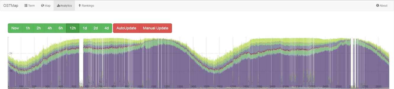
The last two segments Analytics and Rankings are providing an aggreagted view on general information or interesting facts of the collected data. Like the number of tweets of the last hours grouped by the tweet language or the longest distance between two tweets of the same user and so on.
Before it becomes more technical take a look at our small demo.
The Technical View
Technologies
OSTMap uses Apache Flink and Apache Accumulo as backend technologies, AngularJS and Leaflet for the frontend.
Stream Processing
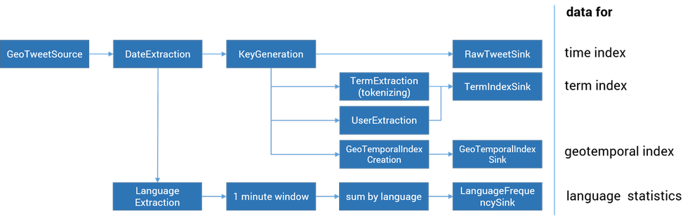
The above figure shows a schematic overview of the stream processing part of OSTMap which was implemented by using the Flink Streaming API. Flink enables us to create several indices on the tweets for fast access in parallel. It reads geo-tagged tweets from Europe and North America from the twitter stream.
The first row of the above figure shows the steps done to create the time index and to store the raw data: a key for the tweet is generated and then written with the tweet itself to Apache Accumulo. In the second and third row the steps done for the term index, which also uses the generated key for cross-table look-ups, are represented. The fourth row builds the geo-temporal index which we will describe later in this article. To create the previously mentioned language frequency we use the tumbling window functionality of Apache Flink. The wokflow is shown in the sixth row.
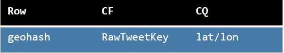
Accumulo Table Design
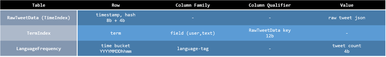
As one can see each tweet is saved in the RawTweetData table with a unique key consisting of the timestamp and hash of the tweet. In addition we added a simple term index pointing to the RawTweetData table for a basic term search. The third table shown in the figure holds information about the language frequencies seen by OSTMap. Further information regarding the data model of Apache Accumulo can be read here: Apache Accumulo data model.
Geotemporal Index
How to map 2d coordinates into 1d key space?
In order to support fast geotemporal queries we use space filling curves. There are many known, for example z curves or geohashes, which we use. In short geohashes are a “hierarchical spatial data structure which subdivides space into buckets of grid shape” (Wikipedia). The length of a given geohash defines its precision. For example: a geohash with length 2 like “d2” covers an area of about 1250km x 625km and a geohash of length 7 like “d2669pz” an area of about 153m x 153m. Locations which are near to each other usually have only small differences in their hashes. Sadly this didn’t hold for all locations.
There are “border” situations where hashes differ strongly from each other. This holds true even when the corresponding locations are next to each other. But this should be no big problem. The calculation of geohashes for given latitude, longitude coordinates is fast with about 3 million GeoHash.encodeHash calls per second on an I7, single thread using the java Geohash library from https://github.com/davidmoten/geo/. The image shows a map covered with (shortened) geohashes and the order they appear as row keys in Apache Accumulo.


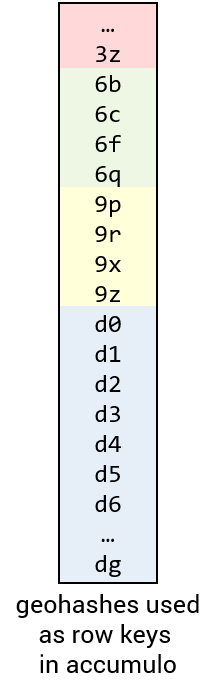
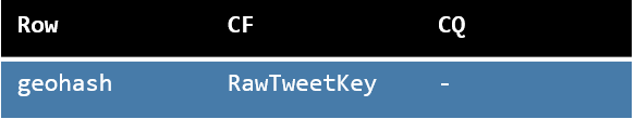
As one can see, regions lying near to each other on the map will be saved near to each other in Apache Accumulo. Since Apache Accumulo is built to support so called “range scans” which means: reading a sequence of data with a given start row until a given end row, it is easy to support queries on data partitioned by geohashes. The Apache Accumulo table holding the geo index would look like this:
How to query a bounding box?
When querying a bounding box we start by calculating the coverage of the box. The result will be a set of geohashes. Those will be used to calculate scan ranges in Apache Accumulo. After the scans are made all data which is not in the bounding box will be dropped by server side iterators and the resulting set of data is returned. The process is visualized in the following image.
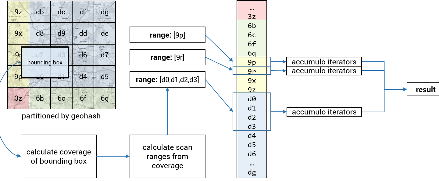
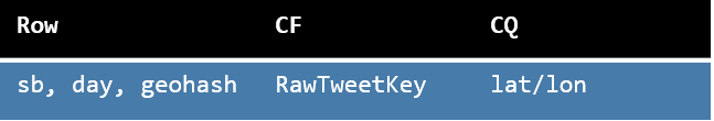
To perform efficient filtering the server side iterators use the lat/lon information given in the column qualifier:
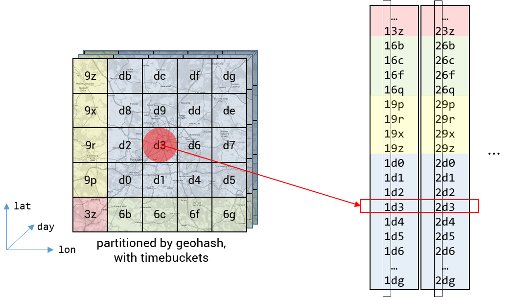
Add the time dimension!
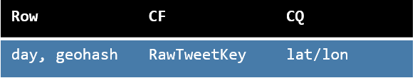
To further increase the query performance we added the time dimension to our table design. We introduced so called “day buckets” in front of our row key. This two byte wide value holds the number of days since first of january 1970. The result are many geospatial indices, one for each day. This enables us to to further shrinken the search space while querying OSTMap.
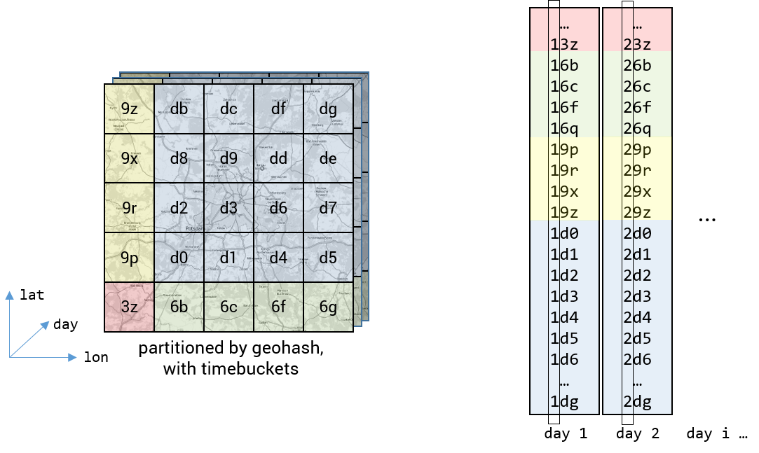
To query a bounding box in this 3-dimensional space one has generate one 2-dimensional geospatial query as shown above for each involved day.
How to deal with hotspots?
This suggestion lacks a method of hotspot mitigation. As shown in the following figure. If there are many data points within one single geohash + time bucket all of these data points are handled by the same node in the cluster, which can lead to high workload for some nodes relative to others.
This issue is easily fixed within the distributed approach by adding a “random” value from 0 to 255 as prefix byte to each row key and a table presplit with 256 splits, one for each value of this so called spreading byte. This leads to a uniform distribution among all involved cluster nodes. From this point on each query will leverage the whole cluster computation power.
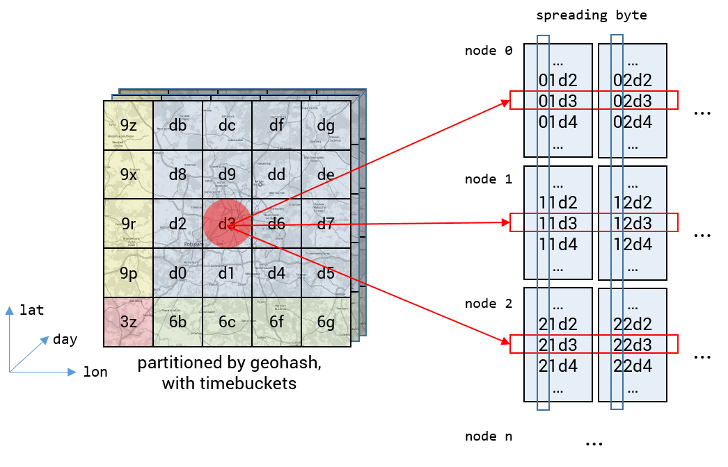
The final design of the geotemporal index table in Apache Accumulo can be seen in the following figure.
Conclusion & Future Work
By using modern technologies and concepts the students managed to create a fast and reliable tweet map in a short time frame. You can even have a look at an excerpt. Possibly we will further enhance the capabilities of OSTMap, especially within the analysis sections.


funded by:

ScaDS.AI Dresden/Leipzig (Center for Scalable Data Analytics and Artificial Intelligence) is a center for Data Science, Artificial Intelligence and Big Data with locations in Dresden and Leipzig.
Dresden
Visitor address
Technische Universität Dresden
ScaDS.AI Dresden/Leipzig
Bürogebäude Strehlener Straße
Strehlener Straße 12, 14
01069 Dresden
ScaDS.AI Dresden/Leipzig
Bürogebäude Strehlener Straße
Strehlener Straße 12, 14
01069 Dresden
Postal address
Technische Universität Dresden
Zentrum für Informationsdienste und Hochleistungsrechnen
ScaDS.AI Dresden/Leipzig
01062 Dresden
Zentrum für Informationsdienste und Hochleistungsrechnen
ScaDS.AI Dresden/Leipzig
01062 Dresden
Leipzig
Visitor address
ScaDS.AI Dresden/Leipzig
Löhrs Carré
Humboldtstraße 25, Uferstr. 11
04105 Leipzig
Löhrs Carré
Humboldtstraße 25, Uferstr. 11
04105 Leipzig
Postal address
Universität Leipzig
Data Science Center ScaDS.AI Leipzig
Internes Postfach: 322001
04081 Leipzig
Data Science Center ScaDS.AI Leipzig
Internes Postfach: 322001
04081 Leipzig
Quicklinks:
Copyright 2026 © SCADS.AI Dresden/Leipzig – All rights reserved.